Decision Trees and Classification Trees

---

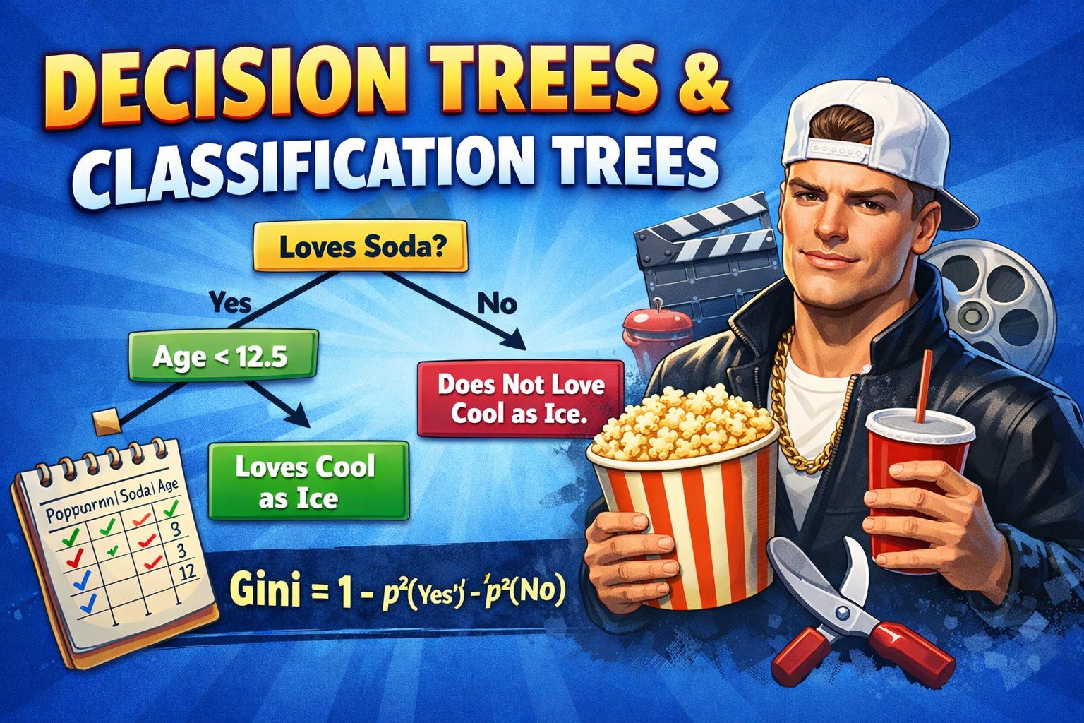
Basic Decision Tree Concepts

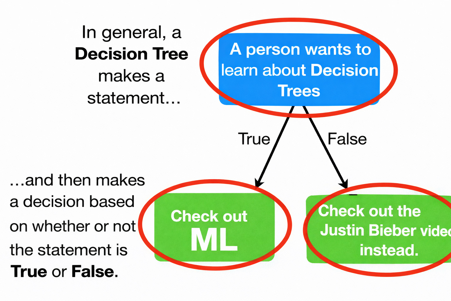
In general, a decision tree makes a statement and then makes a decision based on whether or not that statement is true or false.

When a decision tree classifies things into categories, it is called a classification tree.

When a decision tree predicts numeric values, it is called a regression tree.

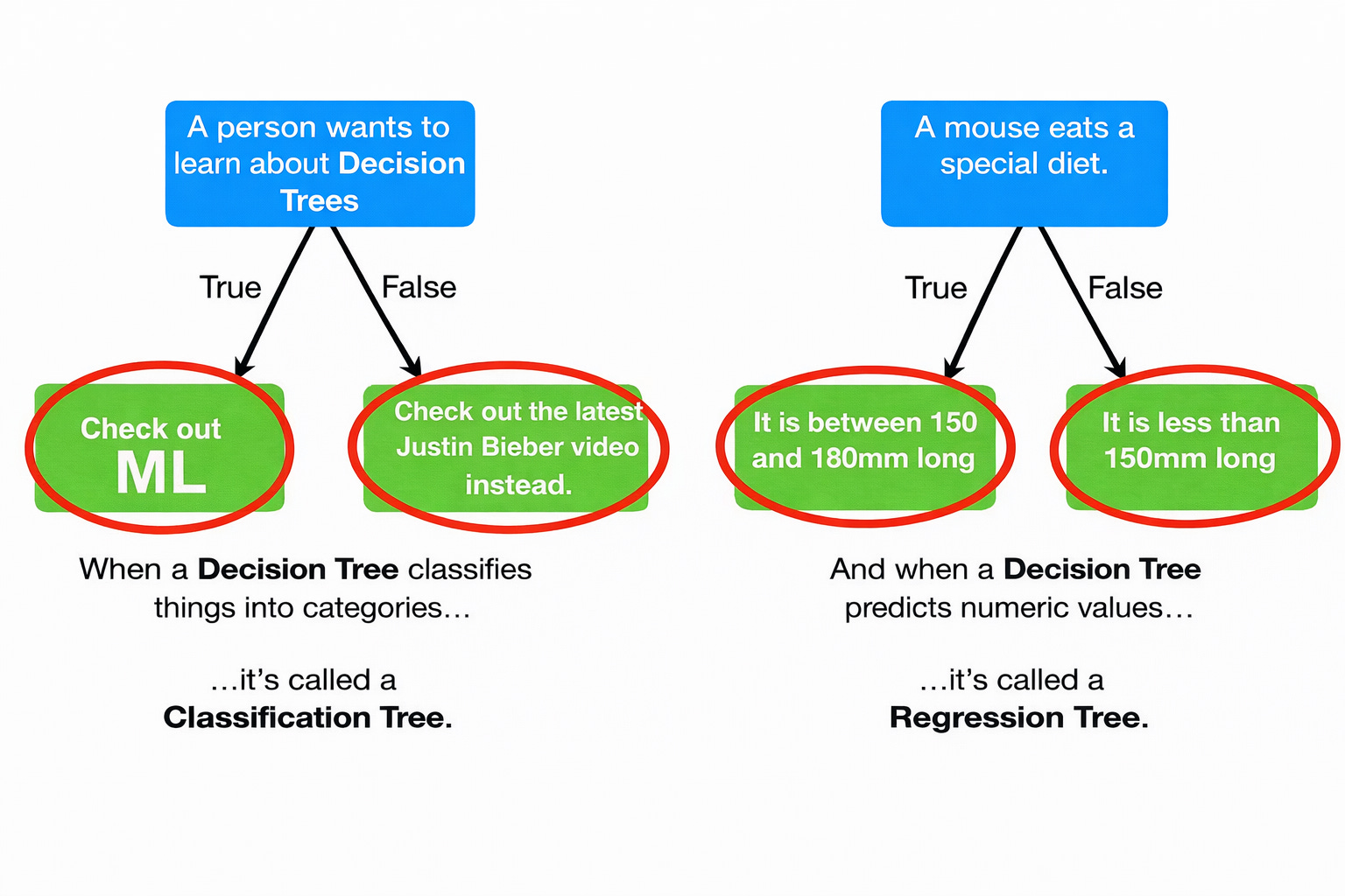
For example, a regression tree might use diet to predict a numeric value for mouse size.

For the remainder of this explanation, the focus is on classification trees.

---

Mixing Data Types

A classification tree can combine:

• Numeric data
• Yes/No data

This means it is possible to mix different data types in the same tree.

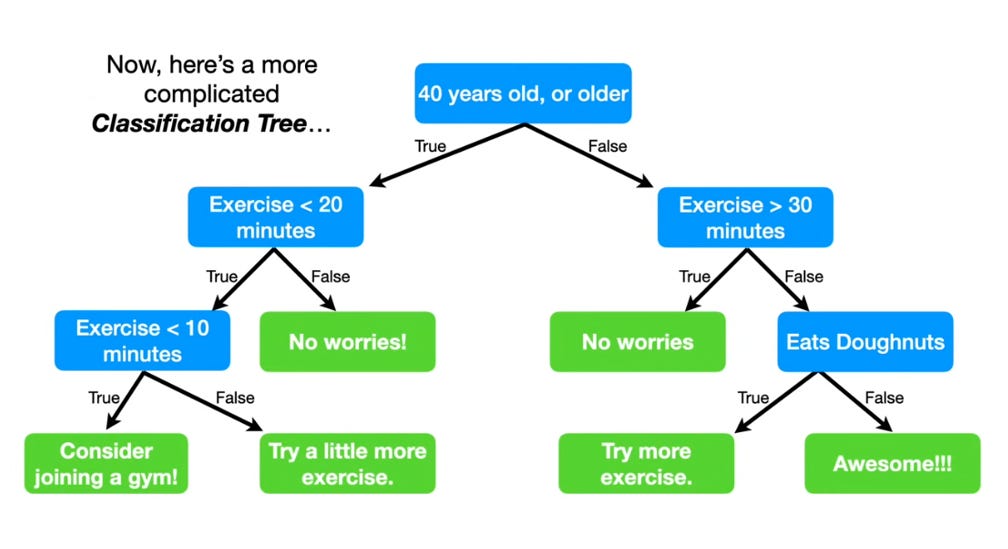
A tree may also ask about the same feature multiple times, and the numeric thresholds used for the same data may be different.

Additionally, the final classifications can be repeated.

---

Using a Classification Tree

Classification trees are generally easy to work with.

To classify something:

1. Start at the top of the tree.
2. Move down the branches.
3. Continue moving until reaching a point where you cannot go any further.
4. That final position determines the classification.

Usually:

• If a statement is true, you go to the left.
• If a statement is false, you go to the right.

Sometimes arrows are labeled True and False, and sometimes they are not.

---

Terminology

Several important technical terms are used in decision trees:

Root Node — The very top of the tree is called the Root Node, or simply the Root.

Internal Nodes / Branches — These are called Internal Nodes or Branches.

Leaf Nodes — The final nodes are called Leaf Nodes, or simply Leaves. Leaves have arrows pointing to them but no arrows pointing away from them.

---

Building a Tree from Raw Data

Now that we know how to use and interpret classification trees, the next step is to learn how to build one from raw data.

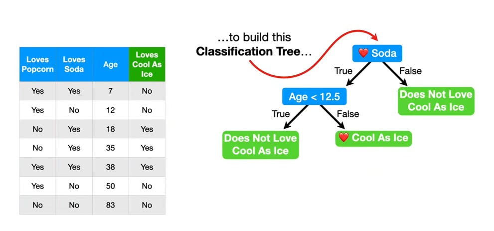
Consider the following dataset. It contains information about several people:

• Whether someone loves popcorn
• Whether someone loves soda
• Their age
• Whether they love the 1991 blockbuster Cool as Ice starring Vanilla Ice

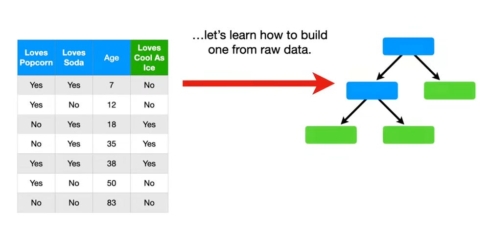
Using this dataset, we want to build a classification tree that predicts whether or not someone loves Cool as Ice.

---

Choosing the Root Question

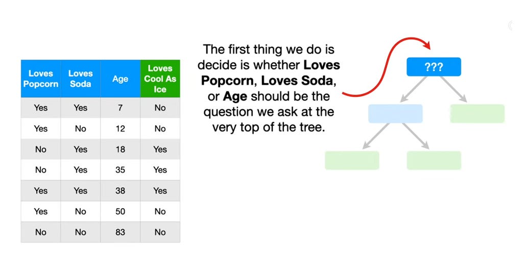
The first step is to determine which feature should appear at the very top of the tree.

The possible options are:

• Loves popcorn
• Loves soda
• Age

To make this decision, we start by examining how well each feature predicts whether someone loves Cool as Ice.

Testing the Feature: Loves Popcorn

To evaluate the feature loves popcorn, we construct a very simple tree that asks only one question:

Does the person love popcorn?

We then run the dataset down this tree.

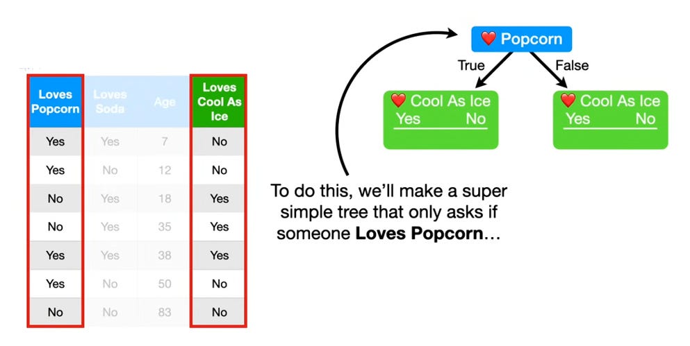
For example:

• The first person loves popcorn, so they go to the leaf on the left. Because they do not love Cool as Ice, we record this by placing 1 under the word "No".
• The second person also loves popcorn, so they also go to the left leaf. Because they also do not love Cool as Ice, we increment "No" to 2.
• The third person does not love popcorn, so they go to the leaf on the right. Because they love Cool as Ice, we record 1 under the word "Yes".

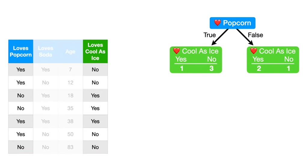
We continue running the remaining rows of the dataset down the tree, keeping track of whether each person loves or does not love Cool as Ice.

Testing the Feature: Loves Soda

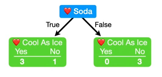
Next, we repeat the exact same process for the feature loves soda.

We build another simple tree that asks:

Does the person love soda?

Then we run the dataset down this tree and record whether each person loves or does not love Cool as Ice in the leaves.

---

Observing the Leaves

After evaluating both trees, we notice something important.

Neither tree does a perfect job predicting who will and who will not love Cool as Ice.

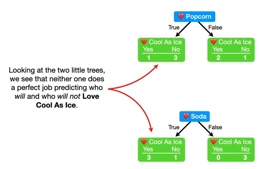
Specifically, three of the leaves contain mixtures of people who do and do not love Cool as Ice. These leaves contain a mixture of classes — because of this mixture, these leaves are called impure leaves.

In contrast, a leaf that contains only one category is called a pure leaf. For example, a leaf that contains only people who do not love Cool as Ice is pure.

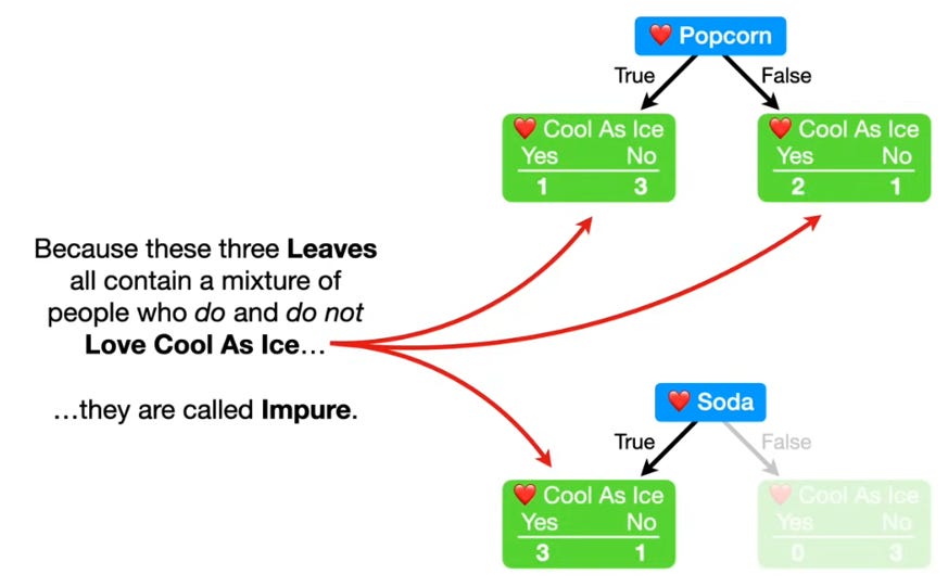
When comparing the two trees:

• Both leaves in the loves popcorn tree are impure
• Only one leaf in the loves soda tree is impure

This suggests that loves soda may be a better predictor. However, instead of relying only on observation, we need a way to quantify the impurity of the leaves — this leads to the concept of Gini Impurity.

---

Quantifying Impurity with Gini Impurity

There are several methods used to measure impurity, including Gini Impurity, Entropy, and Information Gain. In this explanation we focus on Gini Impurity, because it is widely used and relatively straightforward.

Calculating Gini Impurity for the "Loves Popcorn" Tree

The formula for Gini Impurity is:

$\text{Gini} = 1 - P(\text{Yes})^2 - P(\text{No})^2$

Where:

• $P(\text{Yes})$ is the probability that a randomly selected person in the leaf loves Cool as Ice
• $P(\text{No})$ is the probability that a randomly selected person does not love Cool as Ice

Left Leaf — 1 person loves Cool as Ice, 3 do not (total = 4):

$\text{Gini} = 1 - \left(\frac{1}{4}\right)^2 - \left(\frac{3}{4}\right)^2 = 1 - 0.0625 - 0.5625 = 0.375$

Right Leaf — 2 people love Cool as Ice, 1 does not (total = 3):

$\text{Gini} = 1 - \left(\frac{2}{3}\right)^2 - \left(\frac{1}{3}\right)^2 = 1 - \frac{4}{9} - \frac{1}{9} = 0.444$

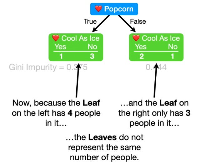
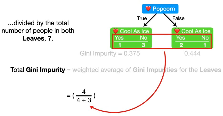
The two leaves contain different numbers of people, so we calculate the total Gini Impurity using a weighted average:

$\text{Weight(left)} = \frac{4}{7}$

$\text{Weight(right)} = \frac{3}{7}$

$\text{Total Gini} = \left(\frac{4}{7} \times 0.375\right) + \left(\frac{3}{7} \times 0.444\right) = 0.405$

Comparing with "Loves Soda"

Using the same process, the Gini Impurity for loves soda is 0.214.

Since lower Gini Impurity means less impurity, loves soda provides a better split than loves popcorn.

---

Numeric and Continuous Variables

So far we calculated Gini Impurity for yes/no features. The feature age contains numeric data, which requires additional steps.

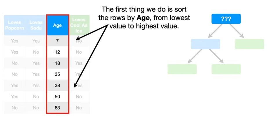
Sorting the Data by Age

The first step is to sort the dataset by age from lowest to highest, to determine possible split points.

Calculating Candidate Thresholds

After sorting the ages, we compute the average age between every pair of adjacent people in the dataset.

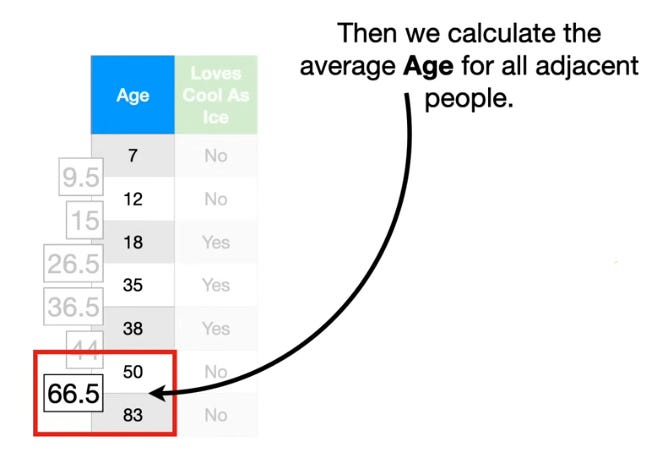
These averages become candidate thresholds. For example:

Is age less than 9.5?

If true, the data goes to the left leaf. If false, it goes to the right leaf.

Example Split: Age < 9.5

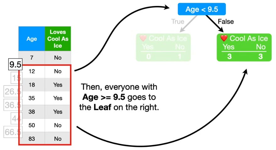
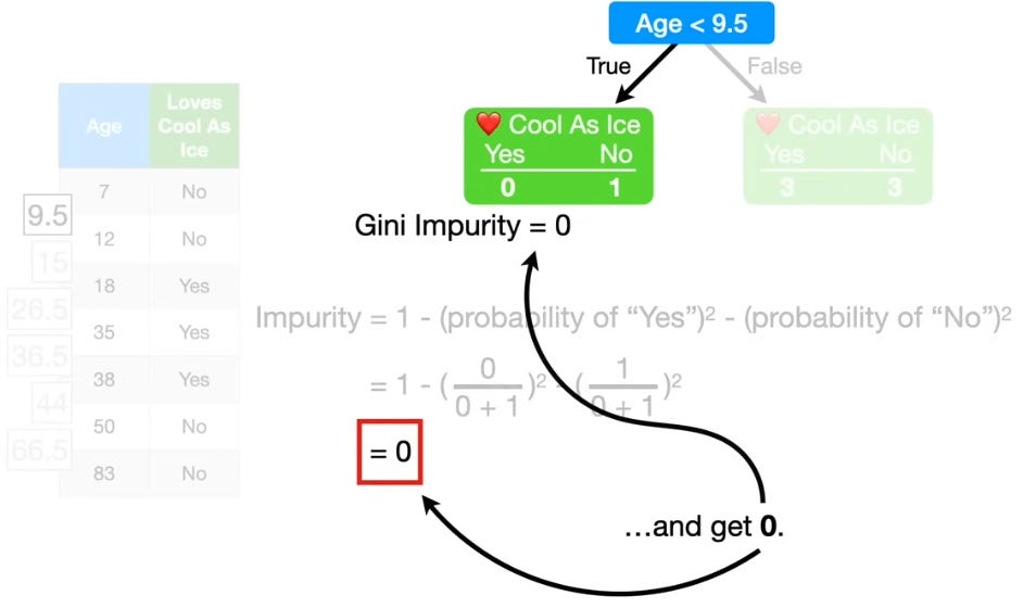
Only one person satisfies this condition. This person does not love Cool as Ice, so the left leaf contains only one category:

• Yes = 0, No = 1

Because every person in this leaf belongs to the same category, the Gini Impurity of the left leaf is 0.

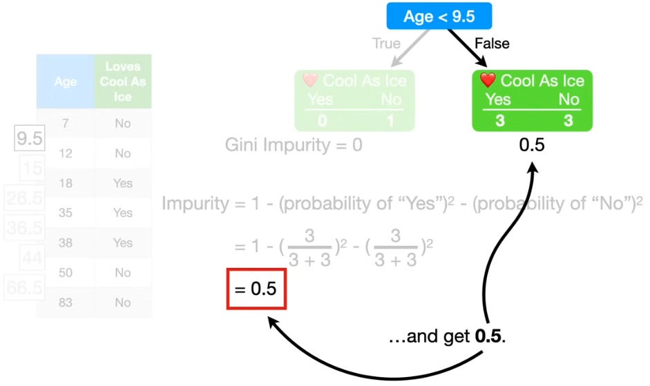
Calculating the Right Leaf

Everyone with Age ≥ 9.5 goes to the right leaf. After calculating the probabilities, the Gini Impurity of the right leaf is 0.5.

After applying the weighted average, the total Gini Impurity for this split is 0.429.

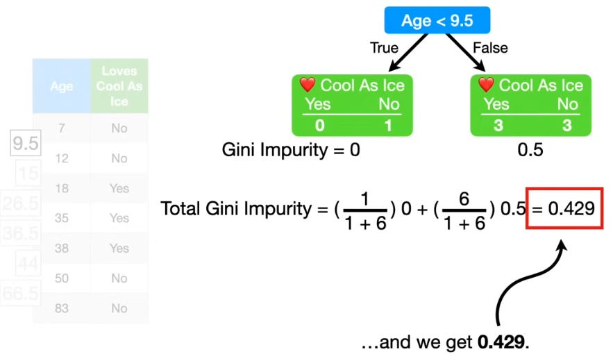
Evaluating All Candidate Thresholds

We repeat this process for all candidate thresholds.

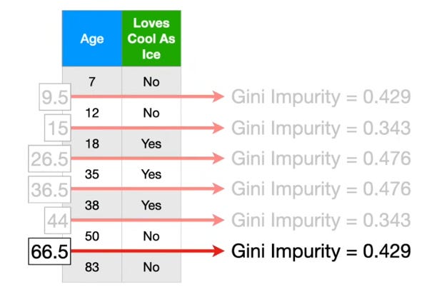
Two candidate thresholds — 15 and 44 — produce the lowest impurity value of 0.343. Since both give the same impurity, either can be chosen. We select Age < 15.

---

Choosing the Root Feature

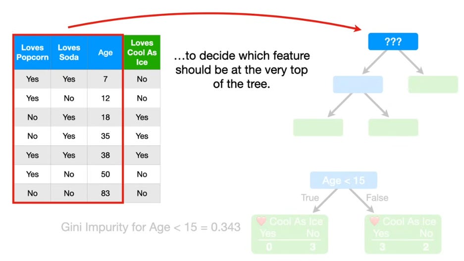
Now we compare the Gini Impurity values for all features:

Feature	Gini Impurity
Loves popcorn	0.405
Loves soda	0.214
Age	0.343

The feature with the lowest Gini Impurity provides the best split. Since loves soda has the lowest impurity, it becomes the root of the classification tree.

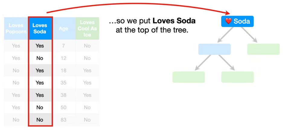
Thus:

• People who love soda go to the left node.
• People who do not love soda go to the right node.

---

Adding Branches

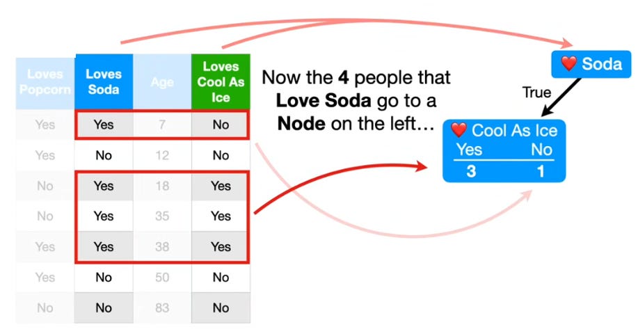
After selecting loves soda as the root, the data splits into two nodes:

• People who love soda → left node (4 people: 3 love Cool as Ice, 1 does not)
• People who do not love soda → right node

Because the left node contains a mixture of classes, it is impure. We attempt to reduce the impurity by splitting it further using:

• Loves popcorn
• Age

Testing the Feature: Loves Popcorn

Among the four people who love soda, two also love popcorn and two do not.

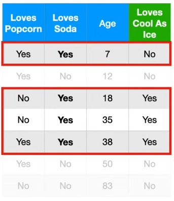
After calculating the impurity of the two leaves and computing the weighted average, the total Gini Impurity for this split is 0.25.

Testing the Feature: Age

We evaluate different age thresholds, but this time only for the people who love soda. The best split found is:

Age < 12.5

This split produces two leaves, both of which contain only one category — so the Gini Impurity is 0.

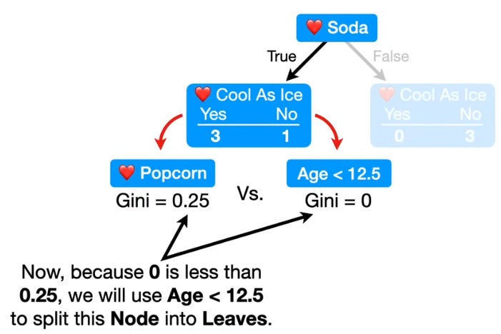
Choosing the Best Split

Split	Gini Impurity
Loves popcorn	0.25
Age < 12.5	0

Since 0 < 0.25, the split using Age < 12.5 is chosen.

---

Adding Leaves

The split using Age < 12.5 produced two new nodes, both containing only one category. Because there is no reason to continue splitting them, these nodes become leaf nodes.

The right node of the root contains the three people who do not love soda — all three do not love Cool as Ice. Since this node is also pure, it becomes a leaf node too.

---

Defining Output Values

After building the structure of the tree, the final step is to assign output values to each leaf node.

In a classification tree, the output value of a leaf is the majority class — the category that appears most frequently in that leaf.

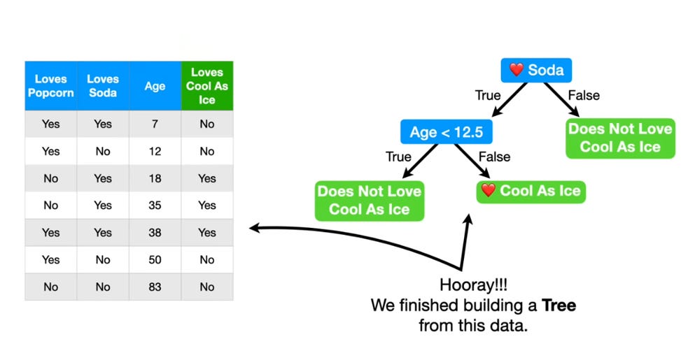
• Leaf 1 — majority do not love Cool as Ice → output: Does not love Cool as Ice
• Leaf 2 — majority love Cool as Ice → output: Loves Cool as Ice

After assigning output values to all leaves, the classification tree is fully constructed and ready to make predictions.

---

Using the Tree

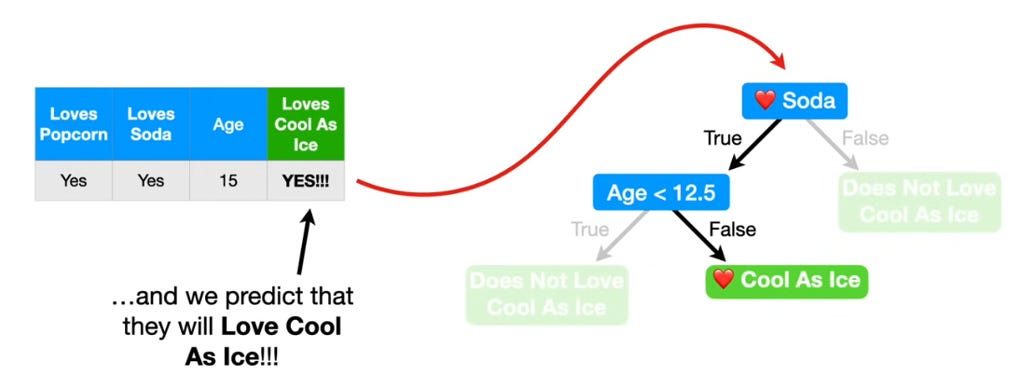
To classify a new example, start at the root node and follow the branches based on whether each condition is true or false.

Example Prediction — a new person who loves soda and is 15 years old:

1. Root: Does the person love soda? → Yes → go left
2. Next: Age < 12.5? → False (age is 15) → go right

Prediction: Loves Cool as Ice

---

How to Prevent Overfitting

When a leaf contains very few data points, it becomes difficult to be confident that the prediction will generalize to new data. This situation can lead to overfitting — when a model fits the training data too closely and fails to generalize.

Method 1: Pruning

Pruning reduces the size of the tree by removing branches that provide little predictive value, improving generalization performance.

Method 2: Limiting Tree Growth

We can require that each leaf must contain a minimum number of data points (e.g., minimum samples per leaf = 3). Some leaves may remain impure, but predictions become more reliable because they are based on more observations.

Using Cross Validation

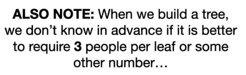
When building a decision tree, we typically do not know the best values for parameters such as the minimum number of samples per leaf or the maximum depth of the tree. To determine the best values, we use cross validation — a technique that tests different parameter settings and selects the one that produces the best predictive performance on validation data.

---

Conclusion

A Decision Tree is a model that makes predictions by evaluating a sequence of conditions and following branches until reaching a leaf node. When the tree predicts categories, it is called a Classification Tree.

The construction of a classification tree involves:

• Selecting the best feature for the root node
• Measuring impurity using Gini Impurity
• Handling numeric and categorical variables
• Splitting nodes to reduce impurity
• Assigning output values to leaf nodes
• Using the tree to classify new data
• Preventing overfitting using pruning and cross validation

By following this process, a classification tree can transform raw data into a predictive model.

---

Further Readings

• Regression Tree

Note: If the term Overfit is new to you, then read Bias and Variance first.

• Prune Regression Tree
• Cross Validation